Variance decomposition

Limix enables flexible fitting of variance component models. Here, we illustrate the usage of variance component models fit to single genes. It is based on the eQTL basics tutorial of limix 1.0, which is now deprecated.

Importing limix

(Source code, png)

The Genetic Model

The model considered by the LIMIX variance decomposition module is an extension of the genetic model employed in standard GWAS, however considers multiple random effects terms:

\[\mathbf{y} = \mathbf{F}\boldsymbol{\alpha} + \sum_{x}\mathbf{u}^{(x)} + \boldsymbol{\psi},\;\;\;\; \mathbf{u}^{(x)}\sim\mathcal{N} \left(\mathbf{0},{\sigma^{(x)}}^2\mathbf{R}^{(x)}\right),\; \boldsymbol{\Psi}\sim\mathcal{N}\left(\mathbf{0},\sigma_e^2\mathbf{I}_N\right)\]

where

\[\begin{split}\begin{eqnarray} \mathbf{y} &=& \text{phenotype vector} \in \mathcal{R}^{N,1} \\ \mathbf{F} &=& \text{matrix of $K$ covariates} \in \mathcal{R}^{N,K} \\ \boldsymbol{\alpha} &=& \text{effect of covariates} \in \mathcal{R}^{K,1} \\ \mathbf{R}^{(x)} &=& \text{is the sample covariance matrix for contribution $x$} \in \mathcal{R}^{N,N} \\ \end{eqnarray}\end{split}\]

If \(\mathbf{R}\) is a genetic contribution from set of SNPs \(\mathcal{S}\), with a bit of abuse of notation we can write \(\mathbf{R}= \frac{1}{C}\mathbf{X}_{:,\,\mathcal{S}}{\mathbf{X}_{:,\,\mathcal{S}}}^T\) where \(C=\frac{1}{N}\text{trace}\left(\mathbf{X}_{:,\,\mathcal{S}_i}{\mathbf{X}_{:,\,\mathcal{S}_i}}^T\right)\).

Limix supports an arbitrary number of fixed or random effects to be included in the model.

Example: cis/trans Variance Decomposition in the glucose condition

Here we use the LIMIX variance decomposition module to quantify the variability in gene expression explained by proximal (cis) and distal (trans) genetic variation. To do so, we build a linear mixed model with a fixed effect intercept, two random effects for cis and trans genetic effects and a noise random effect:

\[\begin{split}\mathbf{y} = \mathbf{1}_N\mu + \mathbf{u}^{(cis)} + \mathbf{u}^{(trans)} + \boldsymbol{\psi},\;\;\;\; \mathbf{u}^{(cis)}\sim\mathcal{N} \left(\mathbf{0},{\sigma^{(x)}}^2\mathbf{R}^{(cis)}\right), \\ \mathbf{u}^{(trans)}\sim \mathcal{N}\left(\mathbf{0},{\sigma^{(x)}}^2\mathbf{R}^{(trans)}\right), \boldsymbol{\Psi}\sim \mathcal{N}\left(\mathbf{0},\sigma_e^2\mathbf{I}_N\right)\end{split}\]

where \(\mathbf{R}^\text{(cis)}\) and \(\mathbf{R}^\text{(trans)}\) are the local and distal relatedeness matrices, built considering all SNPs in cis and trans (i.e., not in cis) respectively. As cis region is defined by the 50kb region around each gene.

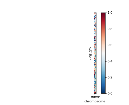
The gene-model is fitted to gene expression in environment 0 for all genes in the Lysine Biosynthesis pathway and variance components are averaged thereafter to obtain pathway based variance components.

(Source code, png)

We then remove the temporary files.

(Source code, png)