eQTL
This tutorial illustrates the use of limix to analyse expression datasets. We consider gene expression levels from a yeast genetics study with freely available data. This data set span 109 individuals with 2,956 marker SNPs and expression levels for 5,493 in glucose and ethanol growth media respectively. It is based on the eQTL basics tutorial of limix 1.0, which is now deprecated.
Importing limix
Downloading data
We are going to use a HDF5 file containg phenotype and genotyped data from a remote repository. Limix provides some handy utilities to perform common command line tasks, like as downloading and extracting files. However, feel free to use whatever method you prefer.
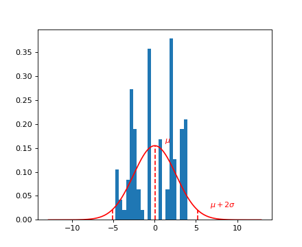
Selecting gene YBR115C under the glucose condition
Query for a specific phenotype, select the phenotype itself, and plot it.
The glucose condition is given by the environment 0.
header = data[‘phenotype’][‘col_header’] query = “gene_ID==’YBR115C’ and environment==0” idx = header.query(query).i.values y = data[‘phenotype’][‘matrix’][:, idx].ravel()
(Source code, png)
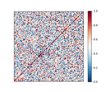
Genetic relatedness matrix
The genetic relatedness will be determined by the inner-product of SNP readings between individuals, and the result will be visualised via heatmap.
(Source code, png)

Univariate association test with linear mixed model
You have the option to either pass a raw array of samples-by-candidates for the association scan or pass a tabular structure naming those candidates. We recommend the second option as it will help maintain the association between the results and the corresponding candidates.
The naming of those candidates is defined here by concatenating the chromossome name and base-pair position. However, it is often the case that SNP IDs are provided along with the data, which can naturally be used for naming those candidates.
(Source code, png)

As you can see, we now have a pandas data frame G that keeps the candidate
identifications together with the actual allele read.
This data frame can be readily used to perform association scan.
(Source code, png)

Inspecting the p-values and effect-sizes are now easier because candidate names are kept together with their corresponding statistics.
(Source code, png)

A Manhattan plot can help understand the result.
(Source code, png)

We then remove the temporary files.
(Source code, png)