Quality control
Box-Cox
-
limix.qc.boxcox(x)[source] Box Cox transformation for normality conformance.
It applies the power transformation
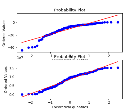
\[\begin{split}f(x) = \begin{cases} \frac{x^{\lambda} - 1}{\lambda}, & \text{if } \lambda > 0; \\ \log(x), & \text{if } \lambda = 0. \end{cases}\end{split}\]to the provided data, hopefully making it more normal distribution-like. The \(\lambda\) parameter is fit by maximum likelihood estimation.
Parameters: X (array_like) – Data to be transformed. Returns: Box Cox transformed data. Return type: array_like Examples
(Source code, png)
Dependent columns
-
limix.qc.remove_dependent_cols(X, tol=1e-06, verbose=False)[source] Remove dependent columns.
Return a matrix with dependent columns removed.
Parameters: X (array_like) – Matrix to might have dependent columns. Returns: Full column rank matrix. Return type: array_like
Genotype
-
limix.qc.indep_pairwise(X, window_size, step_size, threshold, verbose=True)[source] Determine pair-wise independent variants.
Independent variants are defined via squared Pearson correlations between pairs of variants inside a sliding window.
Parameters: - X (array_like) – Sample by variants matrix.
- window_size (int) – Number of variants inside each window.
- step_size (int) – Number of variants the sliding window skips.
- threshold (float) – Squared Pearson correlation threshold for independence.
- verbose (bool) – True for progress information; False otherwise.
Returns: ok
Return type: boolean array defining independent variants
Examples
>>> from numpy.random import RandomState
>>> from limix.qc import indep_pairwise
>>>
>>> random = RandomState(0)
>>> X = random.randn(10, 20)
>>>
>>> indep_pairwise(X, 4, 2, 0.5, verbose=False)
array([ True,  True, False,  True,  True,  True,  True,  True,  True,
        True,  True,  True,  True,  True,  True,  True,  True,  True,
        True,  True])
-
limix.qc.compute_maf(X)[source] Compute minor allele frequencies.
It assumes that
Xencodes 0, 1, and 2 representing the number of alleles (or dosage), orNaNto represent missing values.Parameters: X (array_like) – Genotype matrix. Returns: Minor allele frequencies. Return type: array_like Examples
>>> from numpy.random import RandomState
>>> from limix.qc import compute_maf
>>>
>>> random = RandomState(0)
>>> X = random.randint(0, 3, size=(100, 10))
>>>
>>> print(compute_maf(X))
[0.49  0.49  0.445 0.495 0.5   0.45  0.48  0.48  0.47  0.435]
Impute
-
limix.qc.mean_impute(X)[source] Column-wise impute
NaNvalues by column mean.It works well with Dask array.
Parameters: X (array_like) – Matrix to have its missing values imputed. Returns: Imputed array. Return type: array_like Examples
>>> from numpy.random import RandomState
>>> from numpy import nan, array_str
>>> from limix.qc import mean_impute
>>>
>>> random = RandomState(0)
>>> X = random.randn(5, 2)
>>> X[0, 0] = nan
>>>
>>> print(array_str(mean_impute(X), precision=4))
[[ 0.9233  0.4002]
 [ 0.9787  2.2409]
 [ 1.8676 -0.9773]
 [ 0.9501 -0.1514]
 [-0.1032  0.4106]]
-
limix.qc.count_missingness(X)[source] Count the number of missing values per column.
Returns: Number of missing values per column. Return type: array_like
Kinship
-
limix.qc.normalise_covariance(K, out=None)[source] Variance rescaling of covariance matrix
K.Let \(n\) be the number of rows (or columns) of
Kand let \(m_i\) be the average of the values in the i-th column. Gower rescaling is defined as\[\mathrm K \frac{n - 1}{\text{trace}(\mathrm K) - \sum m_i}.\]It works well with Dask array as log as
outisNone.Notes
The reasoning of the scaling is as follows. Let \(\mathbf g\) be a vector of \(n\) independent samples and let \(\mathrm C\) be the Gower’s centering matrix. The unbiased variance estimator is
\[v = \sum_i \frac{(g_i-\overline g)^2}{n-1} =\frac{\mathrm{Tr} [(\mathbf g-\overline g\mathbf 1)^t(\mathbf g-\overline g\mathbf 1)]} {n-1} = \frac{\mathrm{Tr}[\mathrm C\mathbf g\mathbf g^t\mathrm C]}{n-1}\]Let \(\mathrm K\) be the covariance matrix of \(\mathbf g\). The expectation of the unbiased variance estimator is
\[\mathbb E[v] = \frac{\mathrm{Tr}[\mathrm C\mathbb E[\mathbf g\mathbf g^t]\mathrm C]} {n-1} = \frac{\mathrm{Tr}[\mathrm C\mathrm K\mathrm C]}{n-1}\]assuming that \(\mathbb E[g_i]=0\). We thus divide \(\mathrm K\) by \(\mathbb E[v]\) to achieve the desired normalisation.
Parameters: - K (array_like) – Covariance matrix to be normalised.
- out (array_like, optional) – Result destination. Defaults to
None.
Examples
>>> from numpy import dot, mean, zeros
>>> from numpy.random import RandomState
>>> from limix.qc import normalise_covariance
>>>
>>> random = RandomState(0)
>>> X = random.randn(10, 10)
>>> K = dot(X, X.T)
>>> Z = random.multivariate_normal(zeros(10), K, 500)
>>> print("%.3f" % mean(Z.var(1, ddof=1)))
9.824
>>> Kn = normalise_covariance(K)
>>> Zn = random.multivariate_normal(zeros(10), Kn, 500)
>>> print("%.3f" % mean(Zn.var(1, ddof=1)))
1.008
Normalisation
-
limix.qc.mean_standardize(X, axis=None, out=None)[source] Zero-mean and one-deviation normalisation.
Normalise in such a way that the mean and variance are equal to zero and one. This transformation is taken over the flattened array by default, otherwise over the specified axis. Missing values represented by
NaNare ignored.It works well with Dask array.
Parameters: Returns: Normalized array.
Return type: array_like
Examples
>>> import limix
>>> from numpy import arange, array_str
>>>
>>> X = arange(15).reshape((5, 3))
>>> print(X)
[[ 0  1  2]
 [ 3  4  5]
 [ 6  7  8]
 [ 9 10 11]
 [12 13 14]]
>>> X = limix.qc.mean_standardize(X, axis=0)
>>> print(array_str(X, precision=4))
[[-1.4142 -1.4142 -1.4142]
 [-0.7071 -0.7071 -0.7071]
 [ 0.      0.      0.    ]
 [ 0.7071  0.7071  0.7071]
 [ 1.4142  1.4142  1.4142]]
-
limix.qc.quantile_gaussianize(x)[source] Normalize a sequence of values via rank and Normal c.d.f.
Parameters: x (array_like) – Sequence of values. Returns: Gaussian-normalized values. Return type: array_like Examples
>>> from limix.qc import quantile_gaussianize
>>> from numpy import array_str
>>>
>>> qg = quantile_gaussianize([-1, 0, 2])
>>> print(array_str(qg, precision=4))
[-0.6745  0.      0.6745]